The Laplacian

In Euclidean space, the Laplacian is defined as $\Delta = - \sum_i \partial^2 / \partial(x_i)^2$. The challenge with discretizing the Laplacian is that, the Laplacian takes the second derivative, but the discrete meshes don't have a natural second derivative.

Integration by Parts

One technique is to use integration by parts to lower the order of differentiation: On a manifold $\mathcal{M}$, given functions $f: \mathcal{M} \to \mathbb{R}$ and $g: \mathcal{M} \to \mathbb{R}$,

$\int_\Omega f \Delta g dA = \text{boundary terms} + \int_\Omega \nabla f \cdot \nabla g dA$

This formula coverts an expression that requires the second derivative to an expression that requires only the first derivative. On a discrete mesh, it is easier to cook up basis of functions on discrete mesh that at least have one derivative.

To use integration by parts, we convert a function $f: \mathcal{M} \to \mathbb{R}$ to its dual function $\mathcal{L}_{f}: L^2(\mathcal{M}) \to \mathbb{R}$ by integrating it against a "test" function $g: \mathcal{M} \to \mathbb{R}$:

$\mathcal{L}_{f}[g] = \int_M f(x) g(x) dA(x)$

Note that to evaluate the function $f$ at a point $y$, we just need to use the delta function as the test function,

$\mathcal{L}_{f}[\delta_y] = \int_M f(x) \delta_y(x) dA(x) = f(y)$

In our case, we want to evaluate $\Delta f$ , whose dual is

$\mathcal{L}_{\Delta f}[g] = \int_{\mathcal{M}} g(\mathbf{x}) \Delta f(\mathbf{x}) dA(\mathbf{x}) = \int_{\mathcal{M}} \nabla g(\mathbf{x}) \cdot \nabla f(\mathbf{x}) dA(\mathbf{x}) + \oint_{\partial \mathcal{M}} g(\mathbf{x}) \nabla f(\mathbf{x}) \cdot \mathbf{n}(\mathbf{x}) dl$

where the last expression in the equation is the boundary term, which we can ignore for closed meshes.

Hat Function

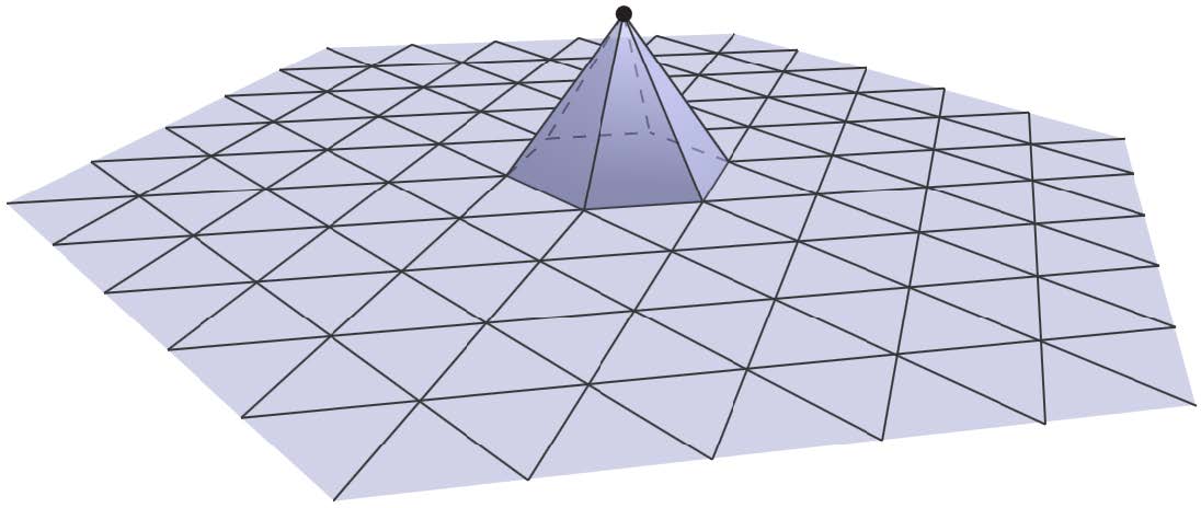
We define a basis of functions $\psi_1(x), \ldots, \psi_k(x): \mathcal{M} \to \mathbb{R}$, where each function $\psi_i(x)$ is a "hat" function centered on vertex $i$ (image of a hat function is shown above, courtsey K. Crane, CMU). Then we can decompose any function $f: \mathcal{M} \to \mathbb{R}$ into $f = \sum_{i=1}^k f_i \psi_i$ by setting $f_i$ to be the value of $f$ at vertex $i$. Intuitively, since a discrete function $f$ is only defined on the vertices, the hat functions $\psi_i$ simply interpolates the value of $f$ on the faces of the triangle mesh in a linear fashion (known as barycentric interpolation).

Discretization

We can evaluate the dual $\mathcal{L}_{\Delta f}$ of the Laplacian $\Delta f$ with a test function $g$ by writing $f$ and $g$ in terms of the basis of the hat function

$\mathcal{L}_{\Delta f}[g] = \sum_{ij} g_i f_j \int_{\mathcal{M}} \Delta \psi_i \cdot \Delta \psi_j \ dA$

Note that, since the gradient of the hat function is constant over a triangle, the dual Laplacian is simply a sum of scalar values (dot products) per face multiplied by the triangle area.

On a triangle with vertex $i$ and edge $e_i$, the gradient $\Delta \psi_i$ is simply $\mathbf{h}_i / ||\mathbf{h}_i||^2$ where $\mathbf{h}_i$ is the height vector normal to the edge $e_i$ and pointing at the vertex $i$.

When $i=j$, the integral $\int \Delta \psi_i \cdot \Delta \psi_j \ dA$ on the triangle with vertex $i$ evaluates to $A ||\nabla \psi_i||^2 = A / ||\mathbf{h}||^2 = (\cot(\alpha) + \cot(\beta))/2$, where $A$ is the area of the triangle and $\alpha$ and $\beta$ are the two angles opposite to the vertex $i$. Then the integral $\int_{\mathcal{M}} \Delta \psi_i \cdot \Delta \psi_i \ dA$ over the entire mesh $\mathcal{M}$ is simply the sum of the integrals over all neighboring triangles $N_k$ of vertex $i$:$\sum_{k \in N_i} \left( \cot \alpha_{ik} + \cot \beta_{ik} \right) / 2$.

When $i \neq j$, the integral $\int \nabla \psi_i \cdot \nabla \psi_j dA$ on the triangle with vertex $i$ and $j$ evaluates to $-(\cot\theta)/2$ where $\theta$ is the angle not on either of the two vertices $i$ and $j$. Then the integral $\int_{\mathcal{M}} \Delta \psi_i \cdot \Delta \psi_j \ dA$ over the entire mesh $\mathcal{M}$ is the sum of integrals over all triangles that incident on edge $e_{ij}$, namely $(\cot \alpha_{ij} + \cot \beta_{ij}) / 2$ where $\alpha_{ij}$ and $\beta_{ij}$ are the angles not on either of the two vertices $i$ and $j$.

Therefore, if we want to evaluate the Laplacian at vertex $i$, we can set the test function to be $\psi_i$, and evaluate the Laplacian $\mathcal{L}_{\Delta f}[\psi_i]$ to be:

$\mathcal{L}_{\Delta f}[\psi_i] = f_i \int_{\mathcal{M}} \nabla \psi_i \cdot \nabla \psi_i \ dA + \sum_{k \in N_i} f_k \int_{\mathcal{M}} \nabla \psi_i \cdot \nabla \psi_k \ dA$

Plugging in the integrals of the hat functions,

$\mathcal{L}_{\Delta f}[\psi_i] = f_i \sum_{k \in N_i} (\cot \alpha_{ik} + \cot \beta_{ik}) / 2 - \sum_{k \in N_i} f_k (\cot\alpha_{ik} + \cot\beta_{ik}) / 2$

We can write this equation in matrix format, $L$, where the $ij$-th entry is

$L_{ij} = \begin{cases} \sum_{k \in N_i} (\cot \alpha_{ik} + \cot \beta_{ik}) / 2 & \text{if } i=j \\ -(\cot\alpha_{ij} + \cot\beta_{ij}) / 2 & \text{if } ij \text{ are adjacent} \\ 0 & \text{otherwise} \end{cases}$

$L$ is known as the discrete cotangent Laplacian matrix.