Laplcian Mesh Fairing

Smoothing operations like mean curvature flow often shrinks the mesh. Therefore, we need to inflate the mesh back to the constrained positions in such a way that preserves the local curvature of the smoothed mesh. The technique we use is based on Olgo-Sorkine's work on Laplacian mesh editing (O. Sorkine et. al. 2004).

We represent each vertex relative to its topological neighbors. This data representation is known as the "Laplacian coordinate", since we effectively represent each vertex as its Laplacian. The main benefit of such representation is that the Laplacian coordinate is intrinsic to the geometry and thus can capture the mesh curvature very well. Moreover, we can easily recover the absolute geometry from Laplacian by solving a sparse linear system, given a set of constrained positions $C$. In particular, we minimize the following energy,

$E(V') = \sum_{i = 1}^n ||\delta_i - L(v'_i)||^2 + \sum_{u_i \in C} ||v'_i - u_i||^2$

by solving the following linear system,

$\begin{bmatrix}L \\ I\end{bmatrix}V'=\begin{bmatrix}\delta\\C\end{bmatrix}$

where $L$ is the Laplacian operator on the mesh, $V'$ is the vertex positions to solve for, and $\delta$ is all vertex Laplacians.

Importantly, the Laplacian coordinate is invariant to translation, but not invariant to scaling and rotation. Our challenge is to find a modification to the classic Laplacian coordinate to make it scale invariant.

The solution is to compute a transformation $T_i$ for each vertex $v_i$ based on the new vertex positions $v_i'$. Then we modify the energy function to be,

$E(V') = \sum_{i = 1}^n ||T_i\delta_i - L(v'_i)||^2 + \sum{u_i \in C} ||v'_i - u_i||^2$

Intuitively, we need to transform the target Laplacian $\delta_i$ to the pose of the neighborhood around vertex $v_i$. In practice, we find the transformation $T_i$ by minimizing the following function,

$\text{argmin}_{T_i} \left(||T_i v_i - v_i'||^2 + \sum_{j \in N_i} ||T_i v_j - v_j'||^2\right)$

where $v_i$ is the initial position of vertex $i$, $v_i'$ is the transformed position of vertex $i$, and $N_i$ is the neighborhood of vertices around $v_i$.

Finally, we model $T_i$ as an affine transformation, such that

$T_i = \begin{bmatrix} s_i & 0 & 0 & t_{i,x} \\ 0 & s_i & 0 & t_{i,y} \\ 0 & 0 & s_i & t_{i,z} \end{bmatrix}$

where $s$ is the scaling factor, and $t_i = (t_{i,x}, t_{i,y}, t_{i,z})$ is the translation vector.

Then we can fit a transformation matrix $T_i$ over the point $v_i$ and its neighbors $N_i$ by solving a linear system, $A_i (s_i, t_i)^T = b_i$ where

$A_i = \begin{bmatrix} v_{k,x} & 1 & 0 & 0 \\ v_{k,y} & 0 & 1 & 0 \\ v_{k,z} & 0 & 0 & 1 \\ \vdots & \vdots & \vdots & \vdots \end{bmatrix}$where $k \in \{i\} \cup N_i$ and

$b_i = \begin{bmatrix} v'_{k,x} \\ v'_{k,y} \\ v'_{k,z} \\ \vdots \end{bmatrix}$

The solution to this linear system gives us a formula $T_i(v'_k)$ to write the transformation matrix $T_i$ in terms of the new vertex positions $v'_{k}$, where $k \in N_i$. We can then use the coefficients of $T_i(v'_k)$ for each vertex $v'_k$ in our energy function $E(V')$ to solve for $T_i$ implicitly.

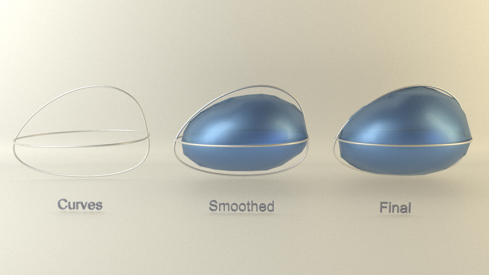
Applying this smoothing algorithm on a simple curve network below, we can see that the final mesh adheres to the constrained positions on the curve network while preserving the curvatures of the smoothed mesh.